Calculating the CIE color of Chlorophyll A and B using Python

A UV-Vis spectrum records how much light a molecule absorbs at each wavelength, but it says nothing about what the molecule actually looks like. Chlorophyll A has absorption peaks near 430 nm and 670 nm — but what color does a solution of it appear to the eye?

Answering that question requires crossing from physics into perception. Color is a sensation produced by the brain’s processing of signals from the retina, not a property of light itself. The same spectral power distribution can look different under different illuminants; different distributions can look identical. This is metamerism: two lights with different spectral compositions produce the same cone responses and appear identical to a normal observer under standard conditions.¹ ²

Psychophysics quantifies this relationship between physical stimuli and perceived sensations. Guy Brindley formalized the distinction in 1970 by categorizing perceptual observations into two types:

Class A observations: Two physically different stimuli are perceived as identical — the observer cannot distinguish them.
Class B observations: All other cases where stimuli are distinguishable.

Color matching is the canonical Class A case. It is also the experimental foundation of the CIE colorimetry system.

The CIE colorimetry system

The CIE colorimetry system, developed by the Commission Internationale d’Éclairage, translates spectral power distributions into standardized color coordinates using color matching experiments.³ ⁴

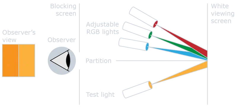
In these experiments, observers view a split field: one half shows a test color, the other a mixture of three primary lights. The observer adjusts the primaries until both halves match. Repeating this across the visible spectrum and averaging over many observers produces a statistical model of human color vision.

CIE color matching experiment. Adapted from literature.

The CIE 1931 model uses additive color mixing based on Color Matching Functions (CMFs), denoted $\bar{x}$ , $\bar{y}$ , and $\bar{z}$ . CMFs are not the spectral sensitivities of the cone cells directly, but linear transformations of them, derived from standardized color matching experiments involving foveal vision, specific field sizes, dark surroundings, and averaged observations from multiple individuals.

By convolution of the sample spectrum $M(\lambda)$ with the CMFs, we calculate tristimulus values $X$ , $Y$ , and $Z$ . These values represent the amounts of the three primary colors (red, green, and blue) required to match the given color.

X = \int_{380}^{780} M(\lambda) \bar{x}(\lambda) \, d\lambda \tag{1}

Y = \int_{380}^{780} M(\lambda) \bar{y}(\lambda) \, d\lambda \tag{2}

Z = \int_{380}^{780} M(\lambda) \bar{z}(\lambda) \, d\lambda \tag{3}

The tristimulus values define a point in a three-dimensional color space. For visualization, this space is reduced to two dimensions using the $x$ and $y$ chromaticity coordinates:

x = \frac{X}{X + Y + Z} \tag{4}

y = \frac{Y}{X + Y + Z} \tag{5}

The $x$ and $y$ coordinates specify a chromaticity (hue and saturation) independently of luminance. This is what makes the diagram useful for comparing colors across different brightness levels.

Python code

Dependencies

The heavy lifting is done by colour-science , a Python library that implements most major colorimetric systems, color space conversions, and color difference metrics. The remaining dependencies are standard: numpy, pandas, and matplotlib. Install them with:

1pip install numpy pandas matplotlib colour-science

Then import them:

1import colour as cl
2import matplotlib.pyplot as plt
3import matplotlib.ticker as tck
4import numpy as np
5import pandas as pd
6
7# Disable some annoying warnings from colour library
8cl.utilities.filter_warnings(colour_usage_warnings=True)

Plot settings

The following settings match the blog’s plot style. If you are following along in a Jupyter notebook, you can skip this block. I use seaborn for its default presets (context, ticks, colorblind palette) and the golden ratio from scipy to set the figure aspect ratio.

 9import seaborn as sns
10from scipy.constants import golden_ratio
11
12# Set seaborn defaults
13sns.set_context("notebook")
14sns.set_style("ticks")
15sns.set_palette("colorblind", color_codes=True)
16
17# Use white color for elements that are typically black
18plt.style.use("dark_background")
19
20# Remove background from figures and axes
21plt.rcParams["figure.facecolor"] = "none"
22plt.rcParams["axes.facecolor"] = "none"
23
24# Default figure size to use throughout
25figure_size = (7, 7 / golden_ratio)

Plotting the CIE (2°) color space

The colour-science library provides a ready-made function for plotting the CIE 1931 chromaticity diagram. The diagram shows all chromaticities visible to a 2° standard observer; the spectral locus traces the monochromatic wavelengths, and any real color falls inside it. We will plot our chlorophyll colors on this diagram later.

26# Instantiate figure and axes
27fig, ax = plt.subplots(1, 1, figsize=(7, 7))
28
29# Plot CIE color space for a 2°
30cl.plotting.plot_chromaticity_diagram_CIE1931(
31    cmfs="CIE 1931 2 Degree Standard Observer",
32    axes=ax,
33    show=False,
34    title=None,
35    spectral_locus_colours="white",
36)
37
38# Axes labels
39ax.set_xlabel("x (2°)")
40ax.set_ylabel("y (2°)")
41
42# Axes limits
43ax.set_xlim(-0.1, 0.85)
44ax.set_ylim(-0.1, 0.95)
45
46# Ticks separation
47ax.xaxis.set_major_locator(tck.MultipleLocator(0.1))
48ax.xaxis.set_minor_locator(tck.MultipleLocator(0.01))
49ax.yaxis.set_major_locator(tck.MultipleLocator(0.1))
50ax.yaxis.set_minor_locator(tck.MultipleLocator(0.01))
51
52# Grid settings
53ax.grid(which="major", axis="both", linestyle="--", color="gray", alpha=0.8)
54
55# Padding adjustment
56plt.tight_layout()
57
58plt.show()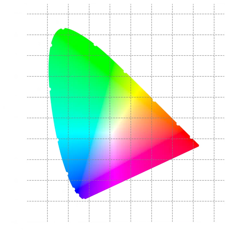

Importing and scaling data

The data are pre-recorded UV-Vis absorption spectra of Chlorophyll A and Chlorophyll B in 70% and 90% acetone solutions, taken from Chazaux et al.⁵ You can download the .csv file as chlorophyll_uv_vis.csv .

59column_names = ["lambda", "chl_a_70", "chl_a_90", "chl_b_70", "chl_b_90"]
60measured_samples = pd.read_csv(
61    "chlorophyll_uv_vis.csv", names=column_names, header=0, index_col="lambda"
62)
63measured_samples

	chl_a_70	chl_a_90	chl_b_70	chl_b_90
lambda
350.0	26132.0	25552.0	29529.0	28301.0
350.4	26251.0	25804.0	29574.0	28114.0
350.8	26666.0	26083.0	29350.0	27946.0
351.2	26703.0	26227.0	29084.0	27660.0
351.6	26834.0	26473.0	28991.0	27632.0
…	…	…	…	…
748.4	-63.0	-269.0	-15.0	-159.0
748.8	-80.0	-289.0	-2.0	-141.0
749.2	-95.0	-283.0	-13.0	-157.0
749.6	-92.0	-292.0	-2.0	-150.0
750.0	82.0	-198.0	69.0	-172.0

1001 rows × 4 columns

Each column records absorbance ( $A$ ) as a function of wavelength ( $\lambda$ ) for one chlorophyll–solvent combination:

60fig, ax = plt.subplots(1, 1, figsize=figure_size)
61
62# Define the labels for the plot's legend
63chl_labels = [
64    "Chlorophyll A (70 % Acetone)",
65    "Chlorophyll A (90 % Acetone)",
66    "Chlorophyll B (70 % Acetone)",
67    "Chlorophyll B (90 % Acetone)",
68]
69
70# Iterate over dataframe and plot each spectrum
71for col, sample_label in zip(measured_samples.columns, chl_labels):
72    ax.plot(measured_samples.index, measured_samples[col], label=sample_label)
73
74# Ticks separation
75ax.xaxis.set_major_locator(tck.MultipleLocator(50))
76ax.xaxis.set_minor_locator(tck.MultipleLocator(10))
77
78# Axes labels
79ax.set_xlabel("Wavelength [nm]")
80ax.set_ylabel("Absorbance [a.u.]")
81
82# Display legend
83ax.legend()
84
85plt.show()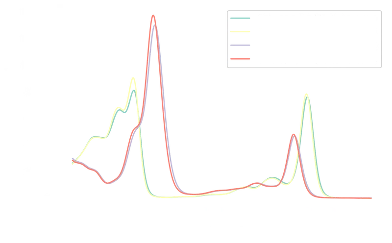

UV-Vis absorption spectra of Chlorophyll A and B in 70% and 90 % acetone
solutions. — UV-Vis absorption spectra of Chlorophyll A and B in 70% and 90 % acetone solutions.

Chlorophyll A absorbs primarily in the blue (~430 nm) and red (~670 nm) regions. Chlorophyll B shows a similar pattern with peaks near 460 nm and 650 nm, its blue peak shifted slightly toward the green. The acetone concentration affects peak intensities but not spectral shape.

Because the four spectra have different absolute absorbance values, we need to normalize them before comparing colors. Normalization discards quantitative information (concentrations), but since our goal is qualitative (what color does each spectrum produce?), this is acceptable.

We use MinMax scaling to map each spectrum to the 0–1 range while preserving its shape:⁶

x_{scaled} = \frac{x - x_{min}}{x_{max} - x_{min}} \tag{6}

A simple custom function avoids pulling in scikit-learn for a one-line operation:

86def normalize(x: pd.Series | np.ndarray) -> pd.Series | np.ndarray:
87    """MinMax scaling from 0 to 1
88
89    Args:
90        x (pd.Series | np.ndarray): series or array to normalize
91
92    Returns:
93        pd.Series | np.ndarray: series or array of normalized values
94    """
95    x_scaled = (x - x.min()) / (x.max() - x.min())
96    return x_scaled

We apply it to the full DataFrame at once, since pandas vectorizes the operation across all columns:

97abs_norm = normalize(measured_samples)
98abs_norm

	chl_a_70	chl_a_90	chl_b_70	chl_b_90
lambda
350.0	0.324398	0.285405	0.227556	0.207087
350.4	0.325869	0.288188	0.227903	0.205727
350.8	0.331001	0.291269	0.226179	0.204505
351.2	0.331458	0.292859	0.224133	0.202425
351.6	0.333078	0.295576	0.223417	0.202221
…	…	…	…	…
748.4	0.000507	0.000254	0.000262	0.000095
748.8	0.000297	0.000033	0.000362	0.000225
749.2	0.000111	0.000099	0.000277	0.000109
749.6	0.000148	0.000000	0.000362	0.000160
750.0	0.002300	0.001038	0.000908	0.000000

1001 rows × 4 columns

A quick plot confirms the spectra now share the same 0–1 scale while retaining their characteristic shapes:

 99fig, ax = plt.subplots(1, 1, figsize=figure_size)
100
101for col, sample_label in zip(abs_norm.columns, chl_labels):
102    ax.plot(abs_norm.index, normalize(abs_norm[col]), label=f"{sample_label} norm")
103
104# Ticks separation
105ax.xaxis.set_major_locator(tck.MultipleLocator(50))
106ax.xaxis.set_minor_locator(tck.MultipleLocator(10))
107ax.yaxis.set_major_locator(tck.MultipleLocator(0.1))
108ax.yaxis.set_minor_locator(tck.MultipleLocator(0.025))
109
110# Axes labels
111ax.set_xlabel("Wavelength [nm]")
112ax.set_ylabel("Absorbance [a.u.]")
113
114# Display legend
115ax.legend()
116
117plt.show()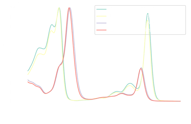

Normalized UV-Vis absorption spectra of Chlorophyll A and B in 70% and 90 %
acetone solutions. — Normalized UV-Vis absorption spectra of Chlorophyll A and B in 70% and 90 % acetone solutions.

Converting absorbance to transmittance

The spectra above record absorbed light. The color we perceive depends on the light that passes through the sample: the transmittance. The conversion from absorbance ( $A$ ) to percent transmittance ( $\%T$ ) follows the Beer-Lambert law:

\%T = 100 \times 10^{-A} = 10^{(2 - A)} \tag{7}

Note that because we are using normalized absorbance values (0–1) rather than actual absorbance, the resulting transmittance values do not represent true physical transmittance. They preserve the spectral shape, which is sufficient for a qualitative color comparison, but should not be interpreted quantitatively.

In code:

120def abs_to_trans(A: pd.Series | np.ndarray) -> pd.Series | np.ndarray:
121    """Convert absorbance to transmittance
122
123    Args:
124        A (pd.Series | np.ndarray): series or array of absorbance values
125
126    Returns:
127        pd.Series | np.ndarray: series or array of transmittance values
128    """
129    T = 10 ** (2 - A)
130    return T

Running it on the normalized absorbance values:

131transm_norm = abs_to_trans(abs_norm)
132transm_norm

	chl_a_70	chl_a_90	chl_b_70	chl_b_90
lambda
350.0	47.380775	51.831637	59.216627	62.074481
350.4	47.220520	51.500565	59.169440	62.269182
350.8	46.665880	51.136488	59.404698	62.444622
351.2	46.616747	50.949585	59.685281	62.744426
351.6	46.443207	50.631871	59.783692	62.773854
…	…	…	…	…
748.4	99.883339	99.941532	99.939788	99.978231
748.8	99.931694	99.992372	99.916775	99.948098
749.2	99.974380	99.977117	99.936247	99.974883
749.6	99.965841	100.000000	99.916775	99.963164
750.0	99.471847	99.761259	99.791184	100.000000

1001 rows × 4 columns

The transmittance spectra, plotted below, should mirror the absorbance spectra inverted:

133fig, ax = plt.subplots(1, 1, figsize=figure_size)
134
135for col, sample_label in zip(transm_norm.columns, chl_labels):
136    ax.plot(transm_norm.index, transm_norm[col], label=f"{sample_label}")
137
138# Ticks separation
139ax.xaxis.set_major_locator(tck.MultipleLocator(50))
140ax.xaxis.set_minor_locator(tck.MultipleLocator(10))
141ax.yaxis.set_major_locator(tck.MultipleLocator(10))
142ax.yaxis.set_minor_locator(tck.MultipleLocator(5))
143
144# Axes labels
145ax.set_xlabel("Wavelength [nm]")
146ax.set_ylabel("Transmittance [%]")
147
148# Display legend
149ax.legend()
150
151plt.show()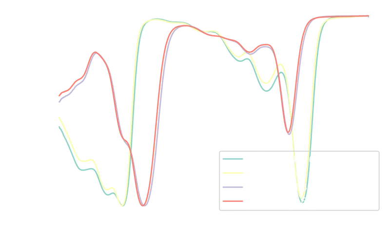

Normalized UV-Vis transmission spectra of Chlorophyll A and B in 70% and 90 %
acetone solutions. — Normalized UV-Vis transmission spectra of Chlorophyll A and B in 70% and 90 % acetone solutions.

The inverse relationship between absorbance and transmittance is visible: peaks in absorbance correspond to troughs in transmittance. A side-by-side comparison:

152fig, ax = plt.subplots(2, 1, sharex=True, figsize=figure_size)
153
154# Iterate over absorbance dataframe
155for col, sample_label in zip(abs_norm.columns, chl_labels):
156    ax[0].plot(abs_norm.index, normalize(abs_norm[col]), label=f"{sample_label}")
157
158# Iterate over transmittance dataframe
159for col, sample_label in zip(transm_norm.columns, chl_labels):
160    ax[1].plot(transm_norm.index, transm_norm[col], label=f"{sample_label}")
161
162# Axes labels
163ax[0].set_ylabel("Absorbance [a.u.]")
164
165ax[1].set_xlabel("Wavelength [nm]")
166ax[1].set_ylabel("Transmittance [%]")
167
168# Ticks separation
169for axis in ax:
170    axis.xaxis.set_major_locator(tck.MultipleLocator(50))
171    axis.xaxis.set_minor_locator(tck.MultipleLocator(10))
172    # Display legend
173    axis.legend()
174
175ax[0].yaxis.set_major_locator(tck.MultipleLocator(0.1))
176ax[0].yaxis.set_minor_locator(tck.MultipleLocator(0.025))
177ax[1].yaxis.set_major_locator(tck.MultipleLocator(10))
178ax[1].yaxis.set_minor_locator(tck.MultipleLocator(5))
179
180plt.show()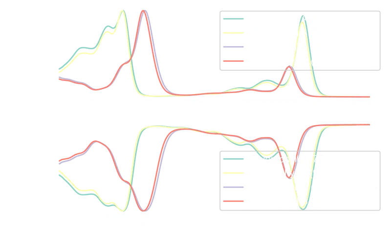

Normalized UV-Vis absorption and transmission spectra of Chlorophyll A and B
in 70% and 90 % acetone solutions. — Normalized UV-Vis absorption and transmission spectra of Chlorophyll A and B in 70% and 90 % acetone solutions.

Calculating the CIE colors

The pipeline for each spectrum:

Build a SpectralDistribution and interpolate to 1 nm intervals (CIE specification).
Compute $XYZ$ tristimulus values with sd_to_XYZ, using the CIE 1931 2° observer CMFs and the D65 daylight illuminant.
Convert $XYZ$ to $xy$ chromaticity coordinates.

The results for absorbance-based and transmittance-based colors are stored in separate lists, then merged into a single DataFrame.

181# Define color matching functions
182cmfs = cl.MSDS_CMFS["cie_2_1931"]
183
184# Define illuminant
185illuminant = cl.SDS_ILLUMINANTS["D65"]
186
187chl_abs_clr = []
188
189# Iterate over each normalized absorbance spectrum
190for col in abs_norm.columns:
191    # Initialize spectral distribution
192    sd = cl.SpectralDistribution(data=abs_norm[col])
193
194    # Interpolate sd to conform to the CIE specifications
195    sd = sd.interpolate(cl.SpectralShape(350, 750, 1))
196
197    # Calculate CIE XYZ coordinates from spectral distribution
198    cie_XYZ = cl.sd_to_XYZ(sd, cmfs, illuminant)
199
200    # Convert to CIE xy coordinates
201    cie_xy = cl.XYZ_to_xy(cie_XYZ)
202
203    # Append the results to the list of sample colors
204    chl_abs_clr.append(
205        {"sample": col, "x_A": np.round(cie_xy[0], 4), "y_A": np.round(cie_xy[1], 4)}
206    )
207
208chl_transm_clr = []
209
210# Iterate over each normalized transmittance spectrum
211for col in transm_norm.columns:
212    # Initialize spectral distribution
213    sd = cl.SpectralDistribution(data=transm_norm[col])
214    sd = sd.interpolate(cl.SpectralShape(350, 750, 1))
215
216    # Calculate CIE XYZ coordinates from spectral distribution
217    cie_XYZ = cl.sd_to_XYZ(sd, cmfs, illuminant)
218
219    # Convert to CIE xy coordinates
220    cie_xy = cl.XYZ_to_xy(cie_XYZ)
221
222    # Append the results to the list of sample colors
223    chl_transm_clr.append(
224        {"sample": col, "x_T": np.round(cie_xy[0], 4), "y_T": np.round(cie_xy[1], 4)}
225    )
226
227# Convert dictionaries to dataframes and join them together
228colors = pd.merge(pd.DataFrame(chl_transm_clr), pd.DataFrame(chl_abs_clr))
229colors

	sample	x_T	y_T	x_A	y_A
0	chl_a_70	0.3046	0.3777	0.2966	0.1330
1	chl_a_90	0.3063	0.3721	0.2948	0.1345
2	chl_b_70	0.3558	0.4365	0.2036	0.0930
3	chl_b_90	0.3538	0.4334	0.2048	0.0904

Visualizing colors on the CIE color space

Plotting the absorbed colors on the CIE 1931 chromaticity diagram:

230# Instantiate figure and axes
231fig, ax = plt.subplots(1, 1, figsize=figure_size)
232
233# Plot CIE color space for a 2°
234cl.plotting.plot_chromaticity_diagram_CIE1931(
235    cmfs="CIE 1931 2 Degree Standard Observer",
236    axes=ax,
237    show=False,
238    title=None,
239    spectral_locus_colours="white",
240)
241
242color_list = ["r", "g", "b", "m"]
243
244for i, c in enumerate(color_list):
245    ax.scatter(
246        colors["x_A"][i],
247        colors["y_A"][i],
248        label=chl_labels[i],
249        color=c,
250        edgecolors="k",
251        alpha=0.8,
252    )
253
254# Axes labels
255ax.set_xlabel("x (2°)")
256ax.set_ylabel("y (2°)")
257
258# Axes limits
259ax.set_xlim(0.18, 0.32)
260ax.set_ylim(0.06, 0.16)
261
262# Ticks separation
263ax.xaxis.set_major_locator(tck.MultipleLocator(0.01))
264ax.xaxis.set_minor_locator(tck.MultipleLocator(0.005))
265ax.yaxis.set_major_locator(tck.MultipleLocator(0.01))
266ax.yaxis.set_minor_locator(tck.MultipleLocator(0.005))
267
268# Grid settings
269ax.grid(which="major", axis="both", linestyle="--", color="gray", alpha=0.8)
270
271# Display legend
272ax.legend()
273
274# Adjust plot padding
275plt.tight_layout()
276
277plt.show()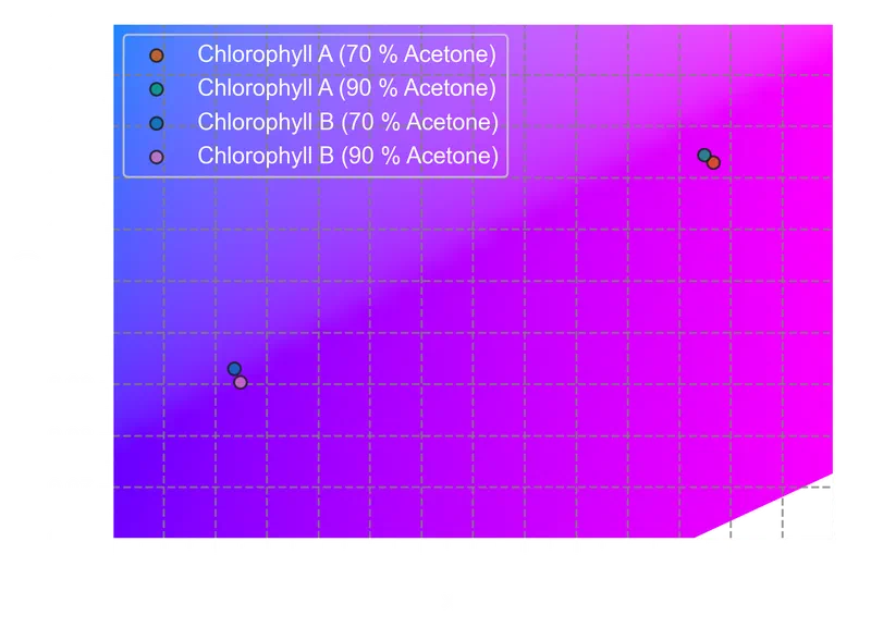

CIE color space for a 2° observer and calculated absorbed colors for
Chlorophyll A and B in 70 % and 90 % acetone with D65
illuminant. — CIE color space for a 2° observer and calculated absorbed colors for Chlorophyll A and B in 70 % and 90 % acetone with D65 illuminant.

The same plot for the transmitted colors:

278# Instantiate figure and axes
279fig, ax = plt.subplots(1, 1, figsize=figure_size)
280
281# Plot CIE color space for a 2°
282cl.plotting.plot_chromaticity_diagram_CIE1931(
283    cmfs="CIE 1931 2 Degree Standard Observer",
284    axes=ax,
285    show=False,
286    title=None,
287    spectral_locus_colours="white",
288)
289
290color_list = ["r", "g", "b", "m"]
291
292for i, c in enumerate(color_list):
293    ax.scatter(
294        colors["x_T"][i],
295        colors["y_T"][i],
296        label=chl_labels[i],
297        color=c,
298        edgecolors="k",
299        alpha=0.8,
300    )
301
302# Axes labels
303ax.set_xlabel("x (2°)")
304ax.set_ylabel("y (2°)")
305
306# Axes limits
307ax.set_xlim(0.25, 0.4)
308ax.set_ylim(0.35, 0.45)
309
310# Ticks separation
311ax.xaxis.set_major_locator(tck.MultipleLocator(0.01))
312ax.xaxis.set_minor_locator(tck.MultipleLocator(0.005))
313ax.yaxis.set_major_locator(tck.MultipleLocator(0.01))
314ax.yaxis.set_minor_locator(tck.MultipleLocator(0.005))
315
316# Grid settings
317ax.grid(which="major", axis="both", linestyle="--", color="gray", alpha=0.8)
318
319# Display legend
320ax.legend(labelcolor="k", edgecolor="k")
321
322# Adjust plot padding
323plt.tight_layout()
324
325plt.show()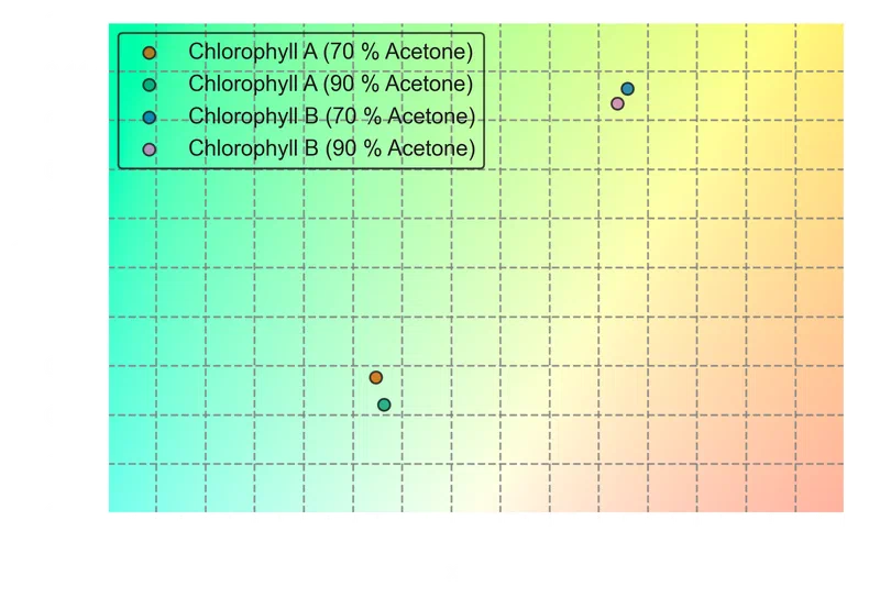

CIE color space for a 2° observer and calculated transmitted colors for
Chlorophyll A and B in 70 % and 90 % acetone with D65
illuminant. — CIE color space for a 2° observer and calculated transmitted colors for Chlorophyll A and B in 70 % and 90 % acetone with D65 illuminant.

The transmitted-color coordinates confirm what the spectra suggest. Both chlorophylls absorb in the blue and red regions and transmit primarily in the green, but the shift in Chlorophyll B’s blue absorption peak toward longer wavelengths pushes its transmitted color toward yellow-green. Chlorophyll A, with its blue peak at shorter wavelengths, sits closer to a neutral green.

Where to go from here

The same pipeline applies to any molecule with a UV-Vis spectrum: dyes, pigments, optical filter glasses, fluorescent proteins. Swapping in the CIE 1976 $L^{*}a^{*}b^{*}$ color space (via colour-science’s XYZ_to_Lab function) would give perceptually uniform coordinates, making it possible to compute meaningful color differences ( $\Delta E$ ) between samples. For quantitative work, the normalization step should be revisited — using actual absorbance values with a defined path length and concentration preserves the physical relationship between Beer-Lambert transmittance and perceived color.

Kingdom, F. A. A.; Prins, N. Psychophysics: A Practical Introduction, 2nd ed.; Academic Press: Amsterdam, NL, 2016; pp. 19–20. https://doi.org/10.1016/C2012-0-01278-1 . ↩︎
Schanda, J. Colorimetry: Understanding the CIE System; John Wiley & Sons: Hoboken, NJ, USA, 2007; pp. 56–59. https://doi.org/10.1002/9780470175637 . ↩︎
Guild, J. The Colorimetric Properties of the Spectrum. Phil. Trans. R. Soc. Lond. A 1931, 230 (681-693), 149–187. https://doi.org/10.1098/rsta.1932.0005 . ↩︎
Smith, T.; Guild, J. The C.I.E. Colorimetric Standards and Their Use. Trans. Opt. Soc. 1931, 33 (3), 73–134. https://doi.org/10.1088/1475-4878/33/3/301 . ↩︎
Chazaux, M.; Schiphorst, C.; Lazzari, G.; Caffarri, S. Precise Estimation of Chlorophyll a , b and Carotenoid Content by Deconvolution of the Absorption Spectrum and New Simultaneous Equations for Chl Determination. Plant J. 2022, 109 (6), 1630–1648. https://doi.org/10.1111/tpj.15643 . ↩︎
Otto, M. Chemometrics: Statistics and Computer Application in Analytical Chemistry, 4th ed.; Wiley-VCH Verlag: Weinheim, DE, 2024; pp. 137–140. https://doi.org/10.1002/9783527843800 . ↩︎

# The CIE colorimetry system

# Python code

# Dependencies

# Plot settings

# Plotting the CIE (2°) color space

# Importing and scaling data

# Converting absorbance to transmittance

# Calculating the CIE colors

# Visualizing colors on the CIE color space

# Where to go from here

The CIE colorimetry system

Python code

Dependencies

Plot settings

Plotting the CIE (2°) color space

Importing and scaling data

Converting absorbance to transmittance

Calculating the CIE colors

Visualizing colors on the CIE color space

Where to go from here